# YAMNet ###### tags: `11th-joint-workshop` * L. Condat, “[A primal–dual splitting method for convex optimization involving lipschitzian, proximable and linear composite terms](https://hal.archives-ouvertes.fr/hal-00609728v5/document),” Journal of Optimization Theory and Applications, vol. 158, 08 2013. * A. G. Howard, M. Zhu, B. Chen, D. Kalenichenko, W. Wang, T. Weyand, M. Andreetto, and H. Adam, “[MobileNets: Efficient Convolutional Neural Networks for Mobile Vision Applications](https://arxiv.org/pdf/1704.04861.pdf),” arXiv e-prints, p. arXiv:1704.04861, Apr 2017. 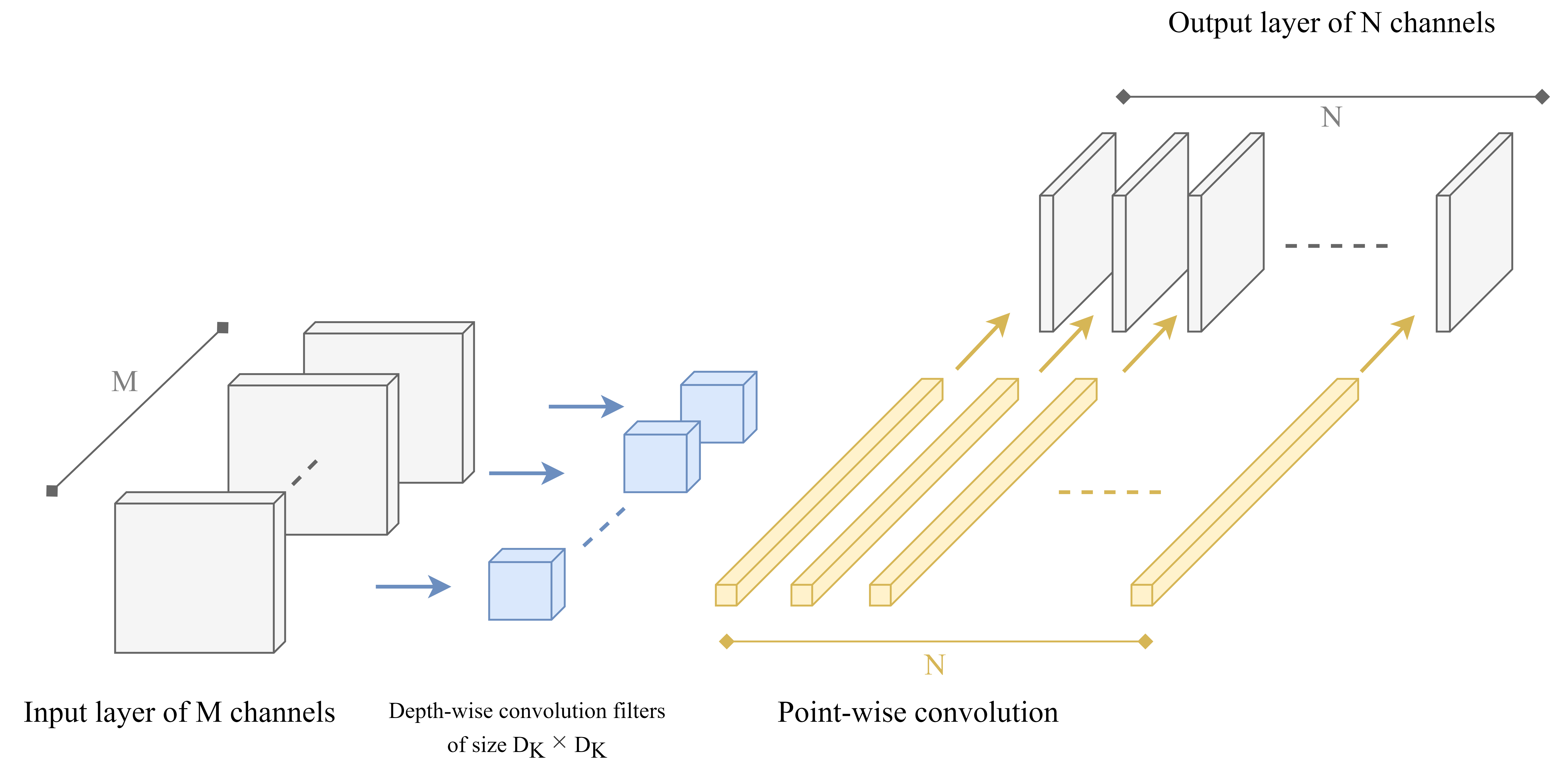## Depthwise Separable Convolution  <center> <i class="fa fa-image"></i> <b>Figure 1</b>: Architecture of Depthwise Separable Convolution </center><br> Depthwise separable convolution is a lightweight form of factorized convolution which factorize a standard convolution into a depthwise convolution and an $1\times 1$ convolution (pointwise convolution, weight factor). Note that the depthwise separable convolution is an incompatible fork of traditional convolution since both sizes of parameters are different, also this factorization is able to accelerate a large amount of computation at a small reduction in accuracy, which will have a more discussion in the following sections. Review on the traditional one, as input a $D_F\times D_F\times M$ feature map $F$ and produces a $D_G\times D_G\times N$ feature map $G$ where $D_F$ is the spatial width and height of a square input feature map, $M$ is the number of input channels, $D_G$ is the spatial width and height of a square output feature map and $N$ is the number of output channel, the standard convolution layer is parameterized by convolution kernel $K$ of size $D_K \times D_K\times M\times N$ where $D_K$ is the dimension of kernel assumed to be square. The output feature map for this approach (with stride 1 and padding) is computed as $$ G_{k, l, n} = \sum_{i,j,m} K_{i, j, m, n} \cdot F_{k+i-1, l+j-1, m} $$ with computational cost being $$ D_K \times D_K \times M \times N \times D_F \times D_F. $$ Depthwise separable convolution are made up of two layers: depthwise convolutions and pointwise convolutions. The depthwise one apply a single filter per each input channel, and the pointwise one produces a simple $1\times 1$ convolution, being used to create a linear combination of the output of the depthwise layer. Depthwise convolution with one filter per input channel can be written as: $$ \hat G_{k, l, m} = \sum_{i, j} \hat K_{i, j, m} \cdot F_{k+i-1, l+j-1, m} $$ where $\hat K$ is the depthwise convolution kernel of size $D_K\times D_K\times M$ and the $m_{th}$ filter of $\hat K$ is applied to the $m_{th}$ channel in $F$. Note that the pointwise convolution is equivalent to the standard convolution of kernel size $1\times 1$. The whole computational cost of the depthwise seperable convolution is $$ D_K \times D_K \times M \times D_F \times D_F + M\times N \times D_F \times D_F, $$ and the number of parameters (without bias vector) is $D_K\times D_K\times M + M\times N$. Table 1 shows a rough comparison between the standard and the separable ones. As $N$ large, the separable <i class="fa fa-table"></i> **Table 1**: Comparison between standard convolution and depthwise separable convolution | | Standard convolution | Separable convolution | Rate (separable / standard) | | ------- | -------------------- | --------------------- | ----------------------------- | | Param # | $D_K^2MN$ | $D_K^2M+MN$ | $\frac{1}{N}+\frac{1}{D_K^2}$ | | Cost | $D_K^2MND_F^2$ | $D_K^2MD_F^2+MND_F^2$ | $\frac{1}{N}+\frac{1}{D_K^2}$ | ## MobileNet The MobileNet structure is built on depthwise separable convolutions except for the first layer which is a standard convolution and the last few layers which are pooling, fully connected layer, and classification. Table 2 shows the architecture of MobileNet, which counts depthwise and pointwise convolutions as separate layers, and each depthwise separable convolution consist of depthwise and pointwise layers followed by batchnrom and ReLU. Note that as $D_K = 3$, MobileNet has about 8 to 9 times less computation than standard convolution for each depthwise separable convolution. <i class="fa fa-table"></i> **Table 2**: MobileNet Body Architecture ($224\times 224\times 3$ for example) | | Type / Stride | Filter Shape | Input Size | | ------:| ------------- | ------------------- | -------------- | | | Conv / s2 | 3 × 3 × 3 × 32 | 224 × 224 × 3 | | | Conv dw / s1 | 3 × 3 × 32 dw | 112 × 112 × 32 | | | Conv / s1 | 1 × 1 × 32 × 64 | 112 × 112 × 32 | | | Conv dw / s2 | 3 × 3 × 64 dw | 112 × 112 × 64 | | | Conv / s1 | 1 × 1 × 64 × 128 | 56 × 56 × 64 | | | Conv dw / s1 | 3 × 3 × 128 dw | 56 × 56 × 128 | | | Conv / s1 | 1 × 1 × 128 × 128 | 56 × 56 × 128 | | | Conv dw / s2 | 3 × 3 × 128 dw | 56 × 56 × 128 | | | Conv / s1 | 1 × 1 × 128 × 256 | 28 × 28 × 128 | | | Conv dw / s1 | 3 × 3 × 256 dw | 28 × 28 × 256 | | | Conv / s1 | 1 × 1 × 256 × 256 | 28 × 28 × 256 | | | Conv dw / s2 | 3 × 3 × 256 dw | 28 × 28 × 256 | | | Conv / s1 | 1 × 1 × 256 × 512 | 14 × 14 × 512 | | (×5) ┌ | Conv dw / s1 | 3 × 3 × 512 dw | 14 × 14 × 512 | | └ | Conv / s1 | 1 × 1 × 512 dw | 14 × 14 × 512 | | | Conv dw / s2 | 3 × 3 × 512 dw | 14 × 14 × 512 | | | Conv / s1 | 1 × 1 × 512 × 1024 | 7 × 7 × 512 | | | Conv dw / s2 | 3 × 3 × 1024 dw | 7 × 7 × 1024 | | | Conv / s1 | 1 × 1 × 1024 × 1024 | 7 × 7 × 1024 | | | Avg Pool / s1 | Pool 7 × 7 | 7 × 7 × 1024 | | | FC / s1 | 1024 × 1000 | 1 × 1 × 1024 | | | Softmax / s1 | Classifier | 1 × 1 × 1000 | ## YAMNet  <center> <i class="fa fa-image"></i> <b>Figure 2</b>: Architecture of YAMNet </center><br> YAMNet is a complete model for audio classification including classification network (employing Mobilnet) and feature extraction. In short, 1. All audio is resampled to 16 kHz mono using `resampy.resample`. 2. A spectrogram is computed using magnitudes `tf.abs` of the Short-Time Fourier Transform (STFT) `tf.signal.stft` with a window size of 25 ms, a window hop of 10 ms, and a periodic Hann window. 3. A mel spectrogram is computed by mapping the spectrogram to 64 mel bins covering the range 125-7500 Hz `tf.signal.linear_to_mel_weight_matrix` 4. A (stablilized) log mel spectrogram is computed by applying $\log (\mathrm{mel\_spectrum}+0.001)$ where the offset $0.001$ is used to avoid taking a logarithm of zero. 5. These features are then framed into 50%-overlapping examples of 0.96 seconds, where each example covers 64 mel bands and 96 frames of 10 ms each. Finally the model for audio classification is revised as <i class="fa fa-table"></i> **Table 3**: YAMNet Body Architecture | | Type / Stride | Filter Shape | Input Size | | ------:| -------------------- | ------------------- | --------------- | | | (Feature extraction) | | | | | Conv / s2 | 3 × 3 × 3 × 32 | 96 × 64 × 1 | | | Conv dw / s1 | 3 × 3 × 32 dw | 48 × 32 × 32 | | | Conv / s1 | 1 × 1 × 32 × 64 | 48 × 32 × 32 | | | Conv dw / s2 | 3 × 3 × 64 dw | 48 × 32 × 64 | | | Conv / s1 | 1 × 1 × 64 × 128 | 24 × 16 × 64 | | | Conv dw / s1 | 3 × 3 × 128 dw | 24 × 16 × 128 | | | Conv / s1 | 1 × 1 × 128 × 128 | 24 × 16 × 128 | | | Conv dw / s2 | 3 × 3 × 128 dw | 24 × 16 × 128 | | | Conv / s1 | 1 × 1 × 128 × 256 | 12 × 8 × 128 | | | Conv dw / s1 | 3 × 3 × 256 dw | 12 × 8 × 256 | | | Conv / s1 | 1 × 1 × 256 × 256 | 12 × 8 × 256 | | | Conv dw / s2 | 3 × 3 × 256 dw | 12 × 8 × 256 | | | Conv / s1 | 1 × 1 × 256 × 512 | 6 × 4 × 512 | | (×5) ┌ | Conv dw / s1 | 3 × 3 × 512 dw | 6 × 4 × 512 | | └ | Conv / s1 | 1 × 1 × 512 dw | 6 × 4 × 512 | | | Conv dw / s2 | 3 × 3 × 512 dw | 6 × 4 × 512 | | | Conv / s1 | 1 × 1 × 512 × 1024 | 3 × 2 × 512 | | | Conv dw / s2 | 3 × 3 × 1024 dw | 3 × 2 × 1024 | | | Conv / s1 | 1 × 1 × 1024 × 1024 | 3 × 2 × 1024 | | | Avg Pool / s1 | Pool 3 × 2 | 3 × 2 × 1024 | | | FC / s1 | 1024 × **521** | 1 × 1 × 1024 | | | Softmax / s1 | Classifier | 1 × 1 × **521** | where output dimension 521 is the number of pruned audio classes based on the ontology of AudioSet. ## Demo